Ttm4110 Ch9 Multimedia Networking
Tags:TTM4110 TTM4110 Chapter 9 - Multimedia Networking
- Streaming stored audio/video
- Conversational voice/audio-over-IP
- Streaming live audio/video
9.1 Multimedia Networking Applications
9.1.1 Properties of Video High bit rate. 100kbps for low quality video conferencing to over 3 Mbps for streaming high-definition movies. Example:
- Photo on facebook average 160kb : 1Kbyte = 8000bits ⇒ 80Mbytes
- Spotify MP3 128kbps encoded ⇒ 64Mbytes
- Video encoded at 2Mbps ⇒ 1Gbyte
- All three 4000 seconds usage time Redundancy: Video compression
- Spatial redundancy, within a given image
- Temporal redundancy: repetition from image to subsequent image
- Use compression to create multiple versions of the same video on different bit rates (can change on the fly like youtube)
9.1.2 Properties of Audio Digital audio, made different from analog audio (which humans hear):
- Analog audio is sampled at some fixed rate (example 8000 samples/s) - Value = real number
- Each of the samples rounded to a finite number of values: Quantization values - a power of two, example 256 quantization values
- Each of the quantization values is represented by a fixed number of bits, bit representation concatenated to form the digital representations of the signal.
- Analog audio signal sampled by 8000 samples/s each quantized by 8 bits, the resulting digital audio will have a rate of 64000 bits per second. Increase sampling rate and number of quantization values → better approximate the original analog signal. Encoding technique: Pulse code modulation (PCM) Speech encoding often uses PCM, of 8000 samples/s and 8bits/sample = 64kbps. CD also use PCM with sampling rate of 44100 samples/s and 16bits/sample = 705kbps for mono and 1411Mbps for stereo.
- Rarely used in the Internet Compression: MPEG 1 layer 3, MP3 (128kbps standard) Advanced Audio Coding (AAC), apple
9.1.3 Types of Multimedia Network Applications
- Streaming stored audio/video
- Conversational voice/audio-over-IP
- Streaming live audio/video
- Streaming stored Audio and Video Combines video and audio components (Spotify) The medium is prerecorded (Movie, TV-show, Youtube and so on) Video placed on servers
- Streaming: Client begins video playout within a few seconds after it begins receiving the video from the server. Client playing the video while receiving later parts. Technique known as streaming, avoids having to download an entire video file.
- Interactivity: Media is prerecorded, user may pause, reposition, forward, backwards, fast-forward and so on through video. Time from when a user makes such a request until the action manifests itself at the client should be less than a few seconds for responsiveness.
- Continuous playout: Once playout begin, proceed according to the original timing of the recording. Data must be received from the server in time for its playout at the client. Otherwise video frame freezing (client waits for delay frame) or frame skipping. Performance: Average throughput, to provide continuous playout, network provides an average throughput to the streaming application that is at least as large the bit rate of the video itself. Using buffering and prefetching.
- Conversational Voice- and Video-over-IP Real-time conversational voice over the Internet referred as Internet telephony - traditional circuit switched telephone service. Commonly called Voice-over-IP (VoIP).
- Timing consideration - audio and video conversational app are highly** delay-sensitive** - few hundred ms (delay > 150ms can’t be heard, 150 - 400 ms is acceptable)
- tolerance of data loss - loss tolerant - occasional glitches can be concealed. Adaptive playout, forward e1Tor correction, and error concealment can mitigate against network-induced packet loss and delay.
- Streaming Live Audio and Video Broadcast radio/tv, transmission on Internet. Live transmission. Done with CDNs, similar to streaming stored media.
9.2 Streaming Stored Video
Placed on servers, users send requests to these servers to view video on demand. Interactable.
- UDP streaming (little used)
- HTTP streaming
- Adaptive HTTP streaming Extensive use of client-side app buffering to mitigate the effect of varying end-to-end delays and available bandwidth between server and client. Tolerate initial delay on video playout, but app buffer can be used as reserve of several seconds. - Client buffering. Absorbs variations in server-to-client delay, if the server-to-client bandwidth briefly drops below the video consumption rate buffer is used. 9.2.1 UDP Streaming
- Server transmit video at a rate the matches the client’s video consumption rate by clocking out the video chunks over UDP at a steady rate.
- Example: Video consumption rate is 2Mbps and each UDP packet carries 8000 bits of video, then server would transmit one UDP packet into its socket every (8000 bits)/(2 Mbps) = 4 msec. UDP doesn’t employ congestion-control mechanism.
- Uses small client-side buffer, big enough to hold less than a second of video
- Before passing video chunk to UDP, server will encapsulate the video chunks within transport packets specially designed for transporting audio and video, using Real Time Transport Protocol (RTP) or similar.
- In addition to server-to-client video stream. The client and server also maintain in parallel, a separate control connection over which the client sends commands regarding session state changes (pause, resume, reposition and so on).
- 3 drawbacks:
- Unpredictable and varying amount of available bandwidth between server and client, constant-rate UDP streaming can fail to provide continuous playout. (Available bandwidth less than video consumption rate.)
- Requires a media control server (RTSP server) to process client-to-server interactivity requests and to track client sate (playpoint). Complexity of deploying large-scale video-on-demand system.
- Firewalls are config to block UDP traffic, prevents users behind these walls to receive UDP video 9.2.2 HTTP Streaming Video stored in an HTTP server as an ordinary file with specific URL. Client establish TCP connection with the server and issues HTTP GET request for that URL. The server then sends the video file, within an HTTP response message, asap as TCP congestion control and flow control will allow.
- On the client side, the bytes are collected in a client app buffer. The number of bytes in this buffer exceeds a predetermined threshold, the client app begins playback.
- Periodically grabs video frames from the client app buffer, decompress the frame and display on user’s screen.
- Server-to-client transmission rate varies due to TCP congestion control mechs. Packets can also be delayed due to TCPs retransmission mechs.
- Use of HTTP over TCP allows the video tr traverse firewalls and NATs more easily, obviates the need for a media control server (RTSP server) reducing cost of large-scale deployment. Youtube and Netflix as example
Prefetching Video
Client-side buffering vary end-to-end delays and varying available bandwidth. Server transmits video at the rate at which the video is to be played out. For streaming stored video, clients attempts to download the video at a rate higher than the consumption rate, thereby prefetching a video frame to be consumed in the future.
Client App buffer and TCP Buffers
Note that if the client application buffer is larger than the video file, then the whole process of moving bytes from the server’s storage to the client’s application buffer is equivalent to an ordinary file download over HTTP-the client simply pulls the video off the server as fast as TCP will allow!
During the pause period, bits are not removed from the client application buffer, even though bits continue to enter the buffer from the server. If the client application buffer is finite, it may eventually become full, which will cause “back pressure” all the way back to the server.
- Specifically, once the client application buffer becomes full, bytes can no longer be removed from the client TCP receive buffer, so it too becomes full. Once the client receive TCP buffer becomes full , bytes can no longer be removed from the server TCP send buffer, so it also becomes full.
- Once the TCP becomes full, the server cannot send any more bytes into the socket.
- Thus, if the user pauses the video, the server may be forced to stop transmitting, in which case the server will be blocked until the user resumes the video.
To determine the resulting rate, note that when the client application removes f bits, it creates room for f bits in the client application buffer, which in turn allows the server to send f additional bits. Thus, the server send rate can be no higher than the video consumption rate at the client. Therefore, a full client application buffer indirectly imposes a limit on the rate that video can be sent from server to client when streaming over HTTP.
Analysis of Video Streaming
As shown in Figure 9.3 , let B denote the size (in bits) of the client’s application buffer, and let Q denote the number of bits that must be buffered before the client application begins playout. (Of course, Q < B.) Let r denote the video consumption rate-the rate at which the client draws bits out of the client application buffer during playback.
- Example, if the video’s frame rate is 30 frames/sec, and each (compressed) frame is 100,000 bits, then r = 3 Mbps. To see the forest through the trees, we’ll ignore TCPs send and receive buffers. Let’s assume that the server sends bits at a constant rate x whenever the client buffer is not full. Suppose at time t = 0, the application buffer is empty and video begins arriving to the client application buffer. We now ask at what time t = t_p does playout begin? And while we are at it, at what time t = t_f does the client application buffer become full?
- First, let’s determine t_ p: the time when Q bits have entered the application buffer and playout begins. Recall that bits arrive to the client application buffer at rate x and no bits are removed from this buffer before playout begins. Thus, the amount of time required to build up Q bits (the initial buffering delay) is t_p = Q/x.
- Now let’s determine** t_f, the point in time when the client application buffer becomes full. We first observe that if **x < r (that is , if the server send rate is less than the video consumption rate), then the client buffer will never become full! Indeed, starting at time t_p, the buffer will be depleted at rate r and will only be filled at rate x < r. Eventually the client buffer will empty out entirely, at which time the video will freeze on the screen while the client buffer waits another** t_p** seconds to build up Q bits of video. Thus, when the available rate in the network is less than the video rate, playout will alternate between periods of continuous playout and periods of freezing.
- In a homework problem, you will be asked to determine the length of each continuous playout and freezing period as a function of Q,** r, and **x .
- Now let’s determine t_f for when x > r. In this case, starting at time t_p, the buffer increases from Q to B at rate x - r since bits are being depleted at rate** r** but are arriving at rate** x** , as shown in Figure 9.3. Given these hints, you will be asked in a homework problem to determine t_f the time the client buffer becomes full._ Note that when the available rate in the network is more than the video rate, after the initial buffering delay, the user will enjoy continuous playout until the video ends._ Early Termination and Repositioning the Video HTTP streaming systems often make use of the HTTP byte-range header in the HTTP GET request message. Useful when user wants to reposition, the client sends a new HTTP request, indicating with the byte-range header from which byte in the file should the server send data. When the server receives the new HTTP request, it can forget about any earlier request and instead send bytes beginning with the byte indicated in the byte-range request.
- For example, suppose that the client buffer is full with B bits at some time t_0 into the video, and at this time the user repositions to some instant t > t_0 + B/r into the video, and then watches the video to completion from that point on. In this case, all B bits in the buffer will be unwatched and the bandwidth and server resources that were used to transmit those B bits have been completely wasted. There is significant wasted bandwidth in the Internet due to early termination, which can be quite costly, particularly for wireless links.
- For this reason, many streaming systems use only a moderate-size client application buffer, or will limit the amount of prefetched video using the byte-range header in HTTP requests.
A third type of streaming is Dynamic Adaptive Streaming over HTTP (DASH) , which uses multiple versions of the video, each compressed at a different rate. DASH is discussed in detail in Section 2.6.2. CDNs are often used to distribute stored and live video. CDNs are discussed in detail in Section 2.6.3.
9.3 Voice-over-IP
Real-time conversational voice over the Internet = Internet telephony =** Voice-over-IP (VoIP)** 9.3.1 Limitation of the Best-Effort IP service The Internet’s network-layer protocol IP provides best-effort service. Service makes its best effort to move each datagram from source to destination as quickly as possible but makes no promises whatsoever about getting the packet to the destination within some delay bound or about a limit on the percentage of packets lost. The lack of such guarantees poses significant challenges to the design of real-time conversational app, sensitive to packet delay, jitter and loss.
- Performance of VoIP over a best-effort network can be enhanced. App-layer techniques.
- The sender generates bytes at a rate of 8000bytes per second; every 20 msecs the sender gathers these bytes into a chunk - encapsulated in a UDP segment via a call to the socket interface.
- Thus, number of bytes in a chunk is (20 msecs)*(8000bytes/s) = 160bytes, and a UDP segment is sent every 20msecs.
- Each packet makes it to the receiver with a constant end-to-end delay, packets receive periodically every 20msecs, Some packets can be lost and most packets will not have the same end-to-end delay.
- Determining (1) when to play back a chunk and (2) what to do with a missing chunk Packet Loss Consider one of the UDP segments generated by VoIP app.
- The UDP segment is encapsulated in an IP datagram, as the datagram wanders through the network, it passes through router buffers (queues) while waiting for transmission on outbound links.
- One or more of the buffers in the path from sender to receiver can be full, in which case the arriving IP datagram may be discarded, never to arrive at the receiving app.
- Loss could be eliminated by sending the packets over TCP (reliable data transfer) rather than over UDP.
- Retransmission mechanism are often considered unacceptable for conversational real-time audio applications such as VoIP, because they increase end-to-end delay.
- TCP congestion control, packet loss may result in a reduction of the TCP sender’s transmission rate to rate that is lower than the receiver’s drain rate, possibly leading to buffer starvation. → Severe impact on voice intelligibility at the receiver.
- Thus UDP is used by default - packet loss between 1 and 20 percent can be tolerated, depending on how voice is encoded and transmitted and how loss is concealed at the receiver.
- Example: Forward error correction (FEC) can help conceal packet loss. Redundant information is transmitted along with the original information so that some of the lost original data can be recovered from the redundant information.
- If one or more of the links between sender and receiver is severely congested, and packet loss exceeds 10 to 20 percent (wireless link) nothing can be done to achieve acceptable audio quality… Limitations… End-to-End Delay
- Is the accumulation of transmission, processing and queuing delays in routers; propagation delays in links; and end-system processing delays.
- For real-time conversational app, such as VoIP, end-to-end delays smaller than 150 msecs are not perceived by a human listener, delays between 150 and 400 msecs can be acceptable but are not ideal; and delays exceeding 400 msecs can seriously hinder the interactivity in voice conversations. Receiving side of a VoIP app will typically disregard any packets that are delayed more than a certain threshold, for example more than 400 msecs. Thus packets that are delayed by more than the threshold are effectively lost. Packet Jitter Crucial component of end-to-end delay is varying queuing delays that a packet experiences in the network’s routers. Because of these varying delays, the time from when a packet is generated at the source until it is received at the receiver can fluctuate from packet to packet. Phenomenon is called jitter.
- Consider two consecutive packets in our VoIP app, sender sends the second packet 20 msecs after sending the first packet, but at the receiver, the spacing between these packets can become greater than 20 msecs.
- To see this, suppose the first packet arrives at a nearly empty queue at a router, but just before the second packet arrives at the queue a large number of packets from other sources arrive at the same queue. Cuz the first packet experiences a small queueing delay and the second packet suffers a large queueing delay at this router, the first and second packets become spaced by more or less than 20 msecs.
- To see this again, consider two consecutive packets, and the second packet arrives at the queue before this first packet is transmitted and before any packets from other sources arrive at the queue. In this case our two packet find themselves one right after the other in the queue. If the time it takes to transmit a packet on the routers outbound link is less than 20 msecs, then the spacing between first and second packets becomes less than 20 msecs. Fortunately, jitter can often be removed by using sequence numbers, timestamps, and a playout delay
9.3.2 Removing Jitter at the Receiver for Audio VoIP app, packets are generated periodically, the receiver attempts periodic playout of voice chunks in the presence of random network jitter. Done by following two mechanism:
- Prepending each chunk with a timestamp. The sender stamps each chunk with the time at which the chunk as generated.
- Delaying playut of chunks at the receiver. As we saw earlier, the playout delay of the received audio chunks must be long enough so that most of the packets are received before their scheduled playout times. This playout delay can either be fixed throughout the duration of the audio session or vary adaptively during the audio session lifetime.
We now discuss how these three mechanisms, when combined, can alleviate or even eliminate the effects of jitter. We examine two playback strategies: fixed playout delay and adaptive playout delay.
- Fixed playout Delay: Strategy where the receiver attempts to play out each chunk exactly q msecs after the chunk is generated. So if a chunk is timestamped at the sender at time t, the receiver plays out the chunk at time t + q, assuming the chunk has arrived by that time. Packets that arrive after scheduled playout times are discarded / lost.
- VoIP can support delays up to about 400 msecs, although a smaller value of q = better call experience.
- If q is made much smaller than 400 msecs, many packets may miss their scheduled playback times due to the network-induced packet jitter.
- Thus if large variations in end-to-end delay are typical, it is preferable to use a large q, but on the other hand, if delay is small and variations in delay are also small, it is preferable to use a small q, even less than 150 msecs.
(The sender generates packets at regular intervals every 20 msecs, the first packet is received at time r, not evenly spaced due to network jitter. The first playout schedule, the fixed initial playout delay is set to p - r, the fourth packet doesn’t arrive by its scheduled playout time, and the receiver considers it lost. For the second playout schedule, the fixed initial playout delay is set to p’ - r. All packets arrive before their schedule playout time, no loss.)
- Adaptive playout Delay Delay-loss trade-off, however for VoIP, long delays can become bothersome if not intolerable. Playout delays ideally be minimized subject to the constraint that the loss be below a few percent. Natural way is to estimate the network delay and the variance of the network delay, and adjust to the playout delay accordingly at the beginning of each talk spurt. Adjusts the playout delays at the beginning of the talk and causes sender’s silent periods to be compressed and elongated (which is not notable in speech (good)).
- Algorithm: Let
The end-to-end network delay of the i-th packet is r_i - t_i due to network jitter. Varies from packet to packet. Let d_i denote an estimate of the average network delay upon reception of the i-th packet:** d_i = (i - u)d_(i-1) + u(r_i - t_i)**
-
U is a fixed constant (example u=0.01), thus** d_i** is a smoothed average of the observed network delays r_i - t_i. Similarly in Round-trip times in TCP. Let v_i denote an estimate of the average deviation of the delay from the estimated average delay:
- The estimates d_i and v_i are calc for / packet received. Determines the playout point for the first packet in any talk spurt. Once having calculated these estimates, the receiver employs algo for the playout of packet, it’s playout time p_i is computed:
- P_i = t_i + d_i + K*v_i (K is a positive constant (ex: K=4))
- The playout point for any subsequent packet in a talk spurt is computed as an offset from the point in time when the first packet in the talk spurt was played out. In particular, let: q_i = p_i - t_i be the length of time from when the first packet in the talk spurt is generated until it is played out. If packet j also belongs to this talk spurt it is played out at time: p_j = t_j + q_i 9.3.3 Recovering from Packet Loss Packet Jitter checked. Preserve acceptable audio quality in the presence of packet loss.Loss recovery schemes. Packet is lost either if it never arrives or if it arrives after its scheduled playout time. Retransmitting a packet that has missed its playout deadline servers no purpose and retransmitting a packet that overflowed a router queue cannot normally be accomplished quickly enough. Thus VoIP app often use loss anticipation schemes: Forward error correction (FEC) and Interleaving
Forward Error Correction (FEC) Add redundant info to the original packet stream. Cost of marginally increasing the transmission rate, the redundant information can be used to reconstruct approx or exact ver of some of the lost packets. 2 simple FEC mechanisms.
- Sends a redundant encoded chunk after every n chunks. The redundant chunk is obtained by exclusively OR-ing the n original n chunks. In this manner if any packet of the group of n+1 packets is lost, the receiver can fully reconstruct the lost packet. But if two or more packets in a group are lost, the receiver cannot reconstruct the lost packages. By keeping n+1, the group size small, a large fraction of the lost packets can be recovered when loss is not excessive. However, the smaller the group size, the greater the relative increase of the transmission rate, by a factor of 1/n. Increases the playout delay too as the receiver must wait to receive the entire group of packets before it can begin playout.
- Send a lower-resolution audio stream as the redundant information. Create both a nominal audio stream and a corresponding low-resolution, low-bit rate audio stream.The low-bit rate stream is referred to as the redundant stream.
Shown in figure, the sender constructs the nth packet by taking the nth chunk from the nominal stream and appending it to the (n-1)th chunk from the redundant stream. This manner, whenever there is noconsecutiive packet loss, the receiver can conceal the loss by playing out the low-bit rate encoded chunk that arrives with the subsequent packet.
- Cope with consecutive loss: simple variation: instead of appending just the (n-1)st low-bit rate chunk to the nth nominal chunk, the sender can append the (n-1)st and (n-2)nd low bit rate chunk, or append the (n-1)st and (n-3)rd low-bit rate chunk, and so on.
- By appending more low-bit rate chunks to each nominal chunk, the audio quality at the receiver becomes acceptable for a wider variety of harsh best-effort environments. On the other hand, the additional chunks increase the transmission bandwidth and the playout delay.
Interleaving
Alternative to transmission, send interleaved audio.
The sender resequences units of audio data before transmission, so that originally adjacent units are separated by a certain distance in the transmitted stream. Interleaving can mitigate the effect of packet losses
- Example: units are 5msecs in length and chunks are 20msecs (4 unit/chunk)
- First chunk contain 1,5,9,13
- Second contain: 2,6,10,14 and so on
- Loss of a single packet from an interleaved stream results in multiple small gaps in the reconstructed stream, as opposed to the single large gap that would occur in a non-interleaved stream.
- Can significantly improve the perceived quality of an audio stream. Low overhead. Disadvantage is that it increases latency. Limits its use for conversational apps such as VoIP, although good for streaming stored audio. Major advantage is that it does not increase the bandwidth requirements of a stream. Error Concealment
- Schemes to attempt to produce a replacement for a lost packet that is similar to the original. Possible since audio signals/speech, exhibit large amounts of short-term self-similarity. As such, these techniques work for relatively small loss rates (less than 15%) and for small packets (4-40msecs). When the loss length approaches the length of a phoneme (5-100msecs) these techniques break down, since the whole phonemes may be missed by the listener.
- Simple form of receiver-based recovery is packet repetition. Replaces lost packets with copies of the packets that arrived immediately before the loss. Low computational complexity and performs reasonably well.
- Another form of receiver-based recovery is interpolation, which uses audio before and after the loss to interpolate a suitable packet to cover the loss. Interpolation performs somewhat better than packet repetition but is significantly more computationally intensive.
9.3.4 Case Study: VoIP with SKYPE Single -
- A popular VoIP app, offers lost of services.
- Skype protocol is proprietary, and it’s control and media packets are encrypted, difficult to know how it operates.
- For both voice and video, Skype clients have at their disposal many different codecs, capable of encoding the media at a wide range of rates and qualities. For example, for as low as 30kbps for a low-quality session up to almost 1Mbps for a high quality session.
- Skype’s audio quality is typically better than POTS (Plain Old Telephone Service) provided by wire-line phone. (Sample voice at 16000 samples/sec or higher vs POTS’ 8000 samples/s)
- Skype sends audio and video packets over UDP by default, but if firewall blocks UDP streams, it uses TCP.
- Uses FEC for loss recovery for both voice and video streams sent over UDP, adapts the audio and video streams it sends to current network conditions by changing video quality and FEC overhead.
- Uses P2P techniques in a number of innovative ways - instant messaging, host-to-host internet telephony - Skype uses it for user location and NAT traversal, organized in hierarchical overlay network, index that maps its peers and super peers.
- P2P also used in Skype relays, establishing calls between hosts in home networks, through NAT by using a super peer which has no NAT block. Multi -
- N > 2 participants, if each user were to send a copy of its audio stream to each of the N-1 other users, then a total of N(N-1) audio streams would need to be sent into the network, to support the audio conference. To reduce this bandwidth usage, Skype employs a clever distribution technique:
- Each user sends its audio stream to the conference initiator, and the conference initiator (host) combines the audio streams into one stream (adding all audio signals together) and then sends a copy of each combined stream to each of the other N-1 participants. Number of streams is thus reduced to 2(N-1).
- For conference video call involving N>2 participants, Skype doesn’t combine the call into one stream at one location and then redistribute the stream to all the participants, as it does for voice calls. Instead each participant’s video stream is routed to a server cluster which in turn relays to each participant the N-1 streams of the N-1 other participants.
- N(N - 1) video streams are being collectively received by the N participants in the conference. The reason is for sending to server instead of each other, because upstream link bandwidths are significantly lower than downstream link bandwidths in most access links, the upstream links may not be able to support the N - 1 streams with the P2P approach.
9.4 Protocols for Real-Time Conversational Applications
Real-time conversational applications, including VoIP and video conferencing, are compelling and very popular. It is therefore not surprising that standards bodies, such as the IETF and ITU, have been busy for many years (and continue to be busy!) at hammering out standards for this class of applications. With the appropriate stand- ards in place for real-time conversational applications, independent companies are creating new products that interoperate with each other. In this section we examine RTP and SIP for real-time conversational applications . Both standards are enjoying widespread implementation in industry products. 9.4.1 RTP
- Used for transporting common audio and video formats. Transporting proprietary sound and video formats. RTP Basics
- Runs on top of UDP, The sending side encapsulates a media chunk within an RTP packet, then encapsulates the packet in a UDP segment, and then hands the segment to IP.
- The receiving side extracts the RTP packet from the UDP segment, then extracts the media chunk from the RTP packet, and then passes the chunk to the media player for decoding and rendering.
- Example: RTP to transport voice.
- Voice source is PCM-encoded (sampled,quantized,digitized) at 64kbps. Suppose app collects the encoded data in 20msecs chunks, rate is 160bytes in a chunk.
- The sending side precedes each chunk of the audio data with an RTP header that includes the type of audio encoding, a seq. Number, and a timestamp. (12 bytes normally). The audio chunk along with the RTP header form the RTP packet, and it is then sent into UDP socket interface.
- At the receiver side, the app receives the RTP packet from its socket interface. Extracts the audio chunk from the RTP packet and uses its header fields to properly decode and play back the audio chunk.
- Easily interoperate with other networked multimedia apps.
- But does not provide any mechanism to ensure timely delivery of data or provide other QoS guarantees.
- Allows each source to be assigned its own independent RTP stream of packet.
-
Not limited to unicast apps, sent over one-to-many and many-to-many multicast trees. RTP session.
RTP Packet Header Fields As shown in Figure 9.8, the four main RTP packet header fields are the payload type, sequence number, timestamp, and source identifier fields.
-
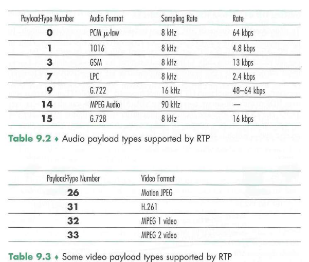
The payload type field in the RTP packet is 7 bits long. For an audio stream, the payload type field is used to indicate the type of audio encoding (for example, PCM, adaptive delta modulation, linear predictive encoding) that is being used. If a sender decides to change the encoding in the middle of a session, the sender can inform the receiver of the change through this payload type field. The sender may want to change the encoding in order to increase the audio quality or to decrease the RTP stream bit rate. Table 9.2 lists some of the audio payload types currently supported by RTP.
-
Sequence number field. The sequence number field is 16 bits long. The sequence number increments by one for each RTP packet sent, and may be used by the receiver to detect packet loss and to restore packet sequence. For example, if the receiver side of the application receives a stream of RTP packets with a gap between sequence numbers 86 and 89, then the receiver knows that packets 87 and 88 are missing. The receiver can then attempt to conceal the lost data
-
Timestamp field. The timestamp field is 32 bits long. It reflects the sampling instant of the first byte in the RTP data packet. As we saw in the preceding section, the receiver can use timestamps to remove packet jitter introduced in the network and to provide synchronous playout at the receiver. The timestamp is derived from a sampling clock at the sender. As an example, for audio the timestamp clock increments by one for each sampling period (for example, each 125 μsec for an 8 kHz sampling clock); if the audio application generates chunks consisting of 160 encoded samples, then the timestamp increases by 160 for each RTP packet when the source is active. The timestamp clock continues to increase at a constant rate even if the source is inactive.
- Synchronization source identifier (SSRC). The SSRC field is 32 bits long. It identifies the source of the RTP stream. Typically, each stream in an RTP session has a distinct SSRC. The SSRC is not the IP address of the sender, but instead is a number that the source assigns randomly when the new stream is started. The probability that two streams get assigned the same SSRC is very small. Should this happen, the two sources pick a new SSRC value
In this application, the sender uses normal RTP and transmits G.722-encoded voice at 48 Kbps. The application collects encoded data in 16 millisecond chunks. Question 1.
- What is the rate at which data is generated at the sender (in bytes)?
- Since the voice is encoded at 48000bps and the application sends the encoded data in 16ms/chunk, the rate at which data is generated at the sender in bytes should be at least 48kbit/s, and the rate per chunk would be (48000bit/s * 0.016s)/8 = 96 bytes.
Question 2.
- What is the size of the IP datagrams sent? You must clearly show the steps in how you calculated your answer and what elements the datagram consists of.
- Since RTP runs on top of UDP, the sending side has to encapsulate the media chunk within an RTP packet then into an UDP segment. The size of the IP datagrams (RTP packet) sent can be calculated with the formula:
- Total packet size = (L2 header: MP or FRF.12 or Ethernet) + (IP/UDP/RTP header) + (voice payload size)
- RTP(usually 12) + UDP(8) + IP(20) overhead = 12+8+20 = 40 bytes
- Voice payload size from question 1 = 96 bytes
- Total packet size must then be at least 40 + 96 = 136 bytes + the Frame(L2) overhead
Question 3.
- Explain how an arbitrary RTP packet in the application will look like. Use actual values from the application when possible. Include the size of the fields and elements of the packet. Loss recovery schemes can be used to preserve acceptable audio quality in the presence of packet loss. We will focus on three types of loss anticipation schemes: forward error correction (FEC) with redundant encoded chunks, FEC with redundant lower-resolution audio stream, and interleaving.
- An arbitrary RTP packet in the application will look like as seen on question 2.
- The RTP header along with the audio chunk form the RTP packet:
- RTP Packet Header: 96 bits (12 bytes)
- (RTP) Version: 2 bits
- Padding: 1 bit
- Extension: 1 bit
- CSRC count: 4 bits
- Marker: 1 bit
- Payload type (indicates the type of encoding): 7 bits
- Sequence Number: 16 bits
- Timestamp: 32 bits
- Synchronization source identifier (SSRC): 32 bits
- Audio Chunk: (96 bytes)
- Using the actual values we get the following: 12 bytes from the RTP header and 96 bytes in an audio chunk, giving us an RTP packet of 108 bytes.
Question 4.
- For each of the three schemes listed in the previous paragraph, show how much additional bandwidth each of them require of our application. For the first type of FEC, suppose a redundant chunk is generated for every five original chunks. For the other type, suppose GSM is used for the low-bit rate encoded stream. For each scheme, include both the new transmission rate and the percentage increase.
- For each of the three schemes listed in the previous paragraph, we can calculate these additional bandwidth each:
- FEC with redundant encoded chunks (every 5 (n+1) original chunks): The new transmission rate is 96+96*1/4 = 120 bytes/chunk which means increase of 25%.
- FEC with redundant lower-resolution audio stream (GSM): (48000+13000bit/s * 0.016s)/8 = 122 bytes/chunk which means increase of 27%.
- Interleaving: only increases the latency from resequencing and reconstructing but doesn’t increase the bandwidth. Thus 96 bytes with the increase of 0%.
Question 5.
- For each of the three schemes, explain what happens if the first packet is lost in every group of five packets. Which scheme will have the better audio quality?
- For each of the three schemes, if the first packet is lost in every group of five packets:
- FEC with redundant encoded chunks (every 5 original chunks): If just the first packet in a group of 5 packets gets lost, it can fully reconstruct the lost packets with the redundant encoded chunk added to the original packet stream, thus the audio quality would be the exact same as if there were no packets lost.
- FEC with redundant lower-resolution audio stream (GSM): Here we refer the nominal stream as the G.722-encoded stream and the low-bit rate GSM as the redundant stream. If the first packet from the nominal stream was to be lost, the lost packet would be constructed by taking it from the redundant stream. Thus in this manner, it is concealed by playing out the low-bit rate encoded chunk that arrives with the subsequent packet. The quality would then be lower than the nominal chunk. But a stream of packets of mostly high-quality chunks and occasional low-quality chunks gives a good quality overall.
- Interleaving: Since the packets are interleaved and a single packet is lost. It would reconstruct the loss packet but there would be multiple small gaps in the reconstructed chunk, lowering the audio quality. It is however better than a single large gap on the first packet.
- From this FEC with redundant encoded chunks will have the best audio quality, GSM and then finally interleaving, assuming only the first packet of every group of five packets is lost.
Question 6.
- Make an illustration of the scenario in question 5 for FEC with redundant encoded chunks. Use the same n value as before. The figure should be made such that it’s clear that you understand how the scheme works.
Question 7.
- For each of the three schemes, explain what happens if the first packet is lost in every group of two packets. Which scheme will have the better audio quality?
- For each of the three schemes, if the first packet is lost in every group of two packets:
- FEC with redundant encoded chunks (every 5 original chunks): Since the first packet is lost in every group of two packets, in n+1 packets we can thus not reconstruct the packets lost. Meaning in every group of n+1 (5) packets, 2 packets is lost and not reconstructed as the FEC packet doesn’t contain enough data. The first packet of every group of two packets would thus be lost.
- FEC with redundant lower-resolution audio stream (GSM): As the answer from question 5, the loss of the first packet is concealed with a low-bit rate encoded chunk taken from the redundant stream. And thus we get a lower audio quality as the packet chunks length are small.
- Interleaving: Since the packets are sent in groups of two packets only. The error concealment of interleaving the stream won’t be that effective as there will be gaps on both the sent packets, lowering the audio quality by a margin.
- From this GSM would have the better audio quality as there won’t be any clipping/gaps of audios, following that is interleaving, since there will be small gaps, but less clipping, small loss rates less than 15% since the application collects encoded data in 16 millisecond chunks. Finally FEC with redundant encoded chunks, where a packet is lost for every group of two packets.
Question 8.
- Make an illustration of the scenario in question 7 for FEC with redundant lowerresolution audio stream. The figure should be made such that it’s clear that the student understands how the scheme works.
Question 9.
- For each of the FEC schemes, how much playback delay does each scheme add? What can be said about the delay of the interleaving scheme?
- For each of the three schemes, the playback delay added for them:
- FEC with redundant encoded chunks (every 5 original chunks): The playback delay added increases by the playout delay, where the time it needs is the enough time to receive all n+1 packets.
- FEC with redundant lower-resolution audio stream (GSM): The receiver receives two packets before playback, thus the increased playout delay is very small.
- Interleaving: The latency would be increased marginally as the packet chunks has to resequence and reconstruct, thus limiting its use for conversational applications.
- From the playback delay of the interleaving scheme we can see that the error concealment works only if the packet chunks are small, but with many units. But on more loss length, the technique will break down and not work that great since the audio’s perceived quality would be very low. Thus it is very unreliable in applications such as VoIP.