Ttm4110 Ch6 The Link Layer
Tags:TTM4110 Chapter 6 : The Link Layer
6.1 Introduction to the link layer
Between the two hosts, datagrams travel over a series of communication links, some wired and some wireless, starting at the source host, passing through a series of packet switches (switches and routers) and ending at the destination host. As we continue down the protocol stack, from the network layer to the link layer, we naturally wonder how packets are sent across the individual links that make up the end-to-end communication path.
- How are the network-layer datagrams encapsulated in the link-layer frames for transmission over a single link?
- Are different link-layer protocols used in the different links along the communication path?
- How are transmission conflicts in broadcast links resolved?
- Is there addressing at the link layer and, if so, how does the link-layer addressing operate with the network-layer addressing we learned about in Chapter 4?
- And what exactly is the difference between a switch and a router?
There are two fundamentally different types of link-layer channels.
- The first type are broadcast channels, which connect multiple hosts in wireless LANs, satellite networks, and hybrid fiber-coaxial cable (HFC) access networks. Since many hosts are connected to the same broadcast communication channel, a so-called medium access protocol is needed to coordinate frame transmission. In some cases, a central controller may be used to coordinate transmissions; in other cases, the hosts themselves coordinate transmissions.
- The second type of link-layer channel is the point-to-point communication link, such as that often found between two routers connected by a long-distance link, or between a user’s office computer and the nearby Ethernet switch to which it is connected. Coordinating access to a point-to-point link is simpler.
We’ll explore several important link-layer concepts and technologies in this chapter. We’ll dive deeper into error detection and correction. We’ll consider multiple access networks and switched LANs, including Ethernet-by far the most prevalent wired LAN technology. We’ll also look at virtual LANs, and data center networks.
Important terminology:
- Refer any device that runs a link-layer (i.e., layer 2) protocol as a node. Nodes include hosts, routers, switches, and WiFi access points.
- Refer to the communication channels that connect adjacent nodes along the communication path as** links**.
For a datagram to be transferred from source host to destination host, it must be moved over each of the individual links in the end-to-end path. Consider sending a datagram from one of the wireless hosts to one of the servers. This datagram will actually pass through six links:
- a WiFi link between sending host and WiFi access point,
- an Ethernet link between the access point and a link-layer switch;
- a link between the link-layer switch and the router,
- a link between the two routers;
- an Ethernet link between the router and a link-layer switch;
- and finally an Ethernet link between the switch and the server.
Over a given link, a transmitting node encapsulates the datagram in a link-layer frame and transmits the frame into the link.
6.1.1 The Services Provided by the Link Layer The basic service of any link layer is to move a datagram from one node to an adjacent node over a single communication link, the details of the provided service can vary from one link-layer protocol to the next. Possible services that can be offered by a link-layer protocol include:
- Framing. Almost all link-layer protocols encapsulate each network-layer datagram within a link-layer frame before transmission over the link. A frame consists of a data field, in which the network-layer datagram is inserted, and a number of header fields. The structure of the frame is specified by the link-layer protocol. We’ll see several different frame formats when we examine specific link-layer protocols in the second half of this chapter.
- Link access. A medium access control (MAC) protocol specifies the rules by which a frame is transmitted onto the link. For point-to-point links that have a single sender at one end of the link and a single receiver at the other end of the link, the MAC protocol is simple (or nonexistent)-the sender can send a frame whenever the link is idle. The more interesting case is when multiple nodes share a single broadcast link-the so-called multiple access problem. Here, the MAC protocol serves to coordinate the frame transmissions of the many nodes.
- Reliable delivery. When a link-layer protocol provides reliable delivery service, it guarantees to move each network-layer datagram across the link without error. Recall that certain transport-layer protocols (such as TCP) also provide a reliable delivery service. Similar to a transport-layer reliable delivery service, a link-layer reliable delivery service can be achieved with acknowledgments and retransmissions (see Section 3.4). A link-layer reliable delivery service is often used for links that are prone to high error rates, such as a wireless link, with the goal of correcting an error locally-on the link where the error occurs-rather than forcing an end-to-end retransmission of the data by a transport- or application-layer protocol. However, link-layer reliable delivery can be considered an unnecessary overhead for low bit-error links, including fiber, coax, and many twisted-pair copper links. For this reason, many wired link-layer protocols do not provide a reliable delivery service.
- Error detection and correction. The link-layer hardware in a receiving node can incor- rectly decide that a bit in a frame is zero when it was transmitted as a one, and vice versa. Such bit errors are introduced by signal attenuation and electromagnetic noise. Because there is no need to forward a datagram that has an error, many link-layer protocols provide a mechanism to detect such bit errors. This is done by having the transmitting node include e1rnr-detection bits in the frame, and having the receiving node perform an error check. Recall from Chapters 3 and 4 that the Internet’s transport layer and network layer also provide a limited form of error detection-the Internet check- sum. Error detection in the link layer is usually more sophisticated and is implemented in hardware. Error correction is similar to error detection, except that a receiver not only detects when bit errors have occurred in the frame but also determines exactly where in the frame the errors have occurred (and then corrects these errors).
6.1.2 Where Is the Link Layer Implemented? Focus on an end system,the link layer is implemented in a router’s line card. But:
- Is a host’s link layer implemented in hardware or software?
- Is it implemented on a separate card or chip, and how does it interface with the rest of a host’s hardware and operating system components?
Figure 6.2 shows a typical host architecture.
- Most part, the link layer is implemented in a network adapter, also sometimes known as a network interface card (NIC).
- At the heart of the network adapter is the link-layer controller, usually a single, special-purpose chip that implements many of the link-layer services (framing, link access, error detection, and so on). Thus, much of a link-layer controller’s functionality is implemented in hardware. Long ago most network adapters were physically separate cards (such as a PCMCIA card or a plug-in card fitting into a PC’s PCI card slot) but increasingly, network adapters are being integrated onto the host’s motherboard-a so-called LAN-on-motherboard configuration.
On the sending side, the controller takes a datagram that has been created and stored in host memory by the higher layers of the protocol stack, encapsulates the datagram in a link-layer frame (filling in the frame’s various fields) , and then transmits the frame into the communication link, following the link-access protocol. On the receiving side, a controller receives the entire frame, and extracts the network layer datagram. If the link layer performs error detection, then it is the sending controller that sets the error-detection bits in the frame header and it is the receiving controller that performs error detection.
- Figure 6.2 shows a network adapter attaching to a host’s bus (e.g., a PCI or PCI-X bus), where it looks much like any other I/O device to the other host components.
- Figure 6.2 also shows that while most of the link layer is implemented in hardware, part of the link layer is implemented in software that runs on the host’s CPU.
- The software components of the link layer implement higher-level link-layer functionality such as assembling link-layer addressing information and activating the controller hardware.
- On the receiving side, link-layer software responds to controller interrupts (e.g., due to the receipt of one or more frames) , handling error conditions and passing a datagram up to the network layer. Thus, the link layer is a combination of hardware and software-the place in the protocol stack where software meets hardware.
6.2 Error-Detection and -Correction Techniques
bit-level error detection and correction - detecting and correcting the corruption of bits in a link-layer frame sent from one node to another physically connected neighboring node-are two services often provided by the link layer.
Error-detection and -correction services are also often offered at the transport layer as well. In this section.
A few of the simplest techniques that can be used to detect and, in some cases, correct such bit errors.

- The receiver’s challenge is to determine whether or not D’ is the same as the original D, given that it has only received D’ and EDC’. The exact wording of the receiver’s decision in Figure 6.3 (we ask whether an error is detected, not whether an error has occurred!) is important. Error-detection and -correction techniques allow the receiver to sometimes, but not always, detect that bit errors have occurred. Even with the use of error-detection bits there still may be undetected bit errors; that is, the receiver may be unaware that the received information contains bit errors. As a consequence, the receiver might deliver a corrupted datagram to the network layer, or be unaware that the contents of a field in the frame’s header has been corrupted.
- We thus want to choose an error-detection scheme that keeps the probability of such occurrences small. Generally, more sophisticated error-detection and-correction techniques (that is, those that have a smaller probability of allowing undetected bit errors) incur a larger overhead-more computation is needed to compute and transmit a larger number of error-detection and -correction bits. Let’s now examine three techniques for detecting errors in the transmitted data-parity checks (to illustrate the basic ideas behind error detection and correction), checksumming methods (which are more typically used in the transport layer), and cyclic redundancy checks (which are more typically used in the link layer in an adapter).
6.2.1 Parity Checks

- In an even parity scheme, the sender simply includes one additional bit and chooses its value such that the total number of ls in the d + 1 bits (the original information plus a parity bit) is even.
- For odd parity schemes, the parity bit value is chosen such that there is an odd number of 1s. Figure 6.4 illustrates an even parity scheme, with the single parity bit being stored in a separate field. Receiver operation is also simple with a single parity bit. The receiver need only count the number of 1s in the received d + 1 bits. If an odd number of 1-valued bits are found with an even parity scheme, the receiver knows that at least one bit error has occurred. More precisely, it knows that some odd number of bit errors have occurred. But what happens if an even number of bit errors occur? You should convince yourself that this would result in an undetected error. If the probability of bit errors is small and errors can be assumed to occur independently from one bit to the next, the probability of multiple bit errors in a packet would be extremely small. In this case, a single parity bit might suffice. However, measurements have shown that, rather than occurring independently, errors are often clustered together in “bursts.” Under burst error conditions, the probability of undetected errors in a frame protected by single-bit parity can approach 50 percent. Clearly, a more robust error-detection scheme is needed (and, fortunately, is used in practice!). But before examining error-detection schemes that are used in practice, let’s consider a simple generalization of one-bit parity that will provide us with insight into error-correction techniques.

- Suppose now that a single bit error occurs in the original d bits of information.
- With this two-dimensional parity scheme, the parity of both the column and the row containing the flipped bit will be in error. The receiver can thus not only detect the fact that a single bit error has occurred, but can use the column and row indices of the column and row with parity errors to actually identify the bit that was corrupted and correct that error! Figure 6.5 shows an example in which the 1-valued bit in position (2,2) is corrupted and switched to a 0-an error that is both detectable and correctable at the receiver. Although our discussion has focused on the original d bits of information, a single error in the parity bits themselves is also detectable and correctable. Two-dimensional parity can also detect (but not correct!) any combination of two errors in a packet.
The ability of the receiver to both detect and correct errors is known as forward error correction (FEC). These techniques are commonly used in audio storage and playback devices such as audio CDs. In a network setting, FEC techniques can be used by themselves, or in conjunction with link-layer ARQ techniques. FEC techniques are valuable because they can decrease the number of sender retransmissions required, more importantly, they allow for immediate correction of errors at the receiver. This avoids having to wait for the round-trip propagation delay needed for the sender to receive a NAK packet and for the retransmitted packet to propagate back to the receiver a potentially important advantage for real-time network applications or links (such as deep-space links) with long propagation delays.
6.2.2 Checksumming Methods In checksumming techniques, the d bits of data in Figure 6.4 are treated as a sequence of k-bit integers.** One simple checksumming method is to simply sum these k-bit integers and use the resulting sum as the error-detection bits. The **Internet checksum is based on this approach-bytes of data are treated as 16-bit integers and summed. The complement of this sum then forms the Internet checksum that is carried in the segment header. The receiver checks the checksum by taking the 1s complement of the sum of the received data (including the checksum) and checking whether the result is all 1 bits. If any of the bits are 0, an error is indicated. In IP the checksum is computed over the IP header (since the UDP or TCP segment has its own checksum). In other protocols, for example, XTP, one checksum is computed over the header and another checksum is computed over the entire packet.
Checksumming methods require relatively little packet overhead. For example, the checksums in TCP and UDP use only 16 bits. However, they provide relatively weak protection against errors as compared with cyclic redundancy check, which is often used in the link layer.
- Why is checksumming used at the transport layer and cyclic redundancy check used at the link layer? Recall that the transport layer is typically implemented in software in a host as part of the host’s operating system. Because transport-layer error detection is implemented in software, it is important to have a simple and fast error-detection scheme such as checksumming. On the other hand, error detection at the link layer is implemented in dedicated hardware in adapters, which can rapidly perform the more complex CRC operations.
6.2.3 Cyclic Redundancy Check (CRC) An error-detection technique used widely in today’s computer networks is based on cyclic redundancy check (CRC) codes. CRC codes are also known as polynomial codes, since it is possible to view the bit string to be sent as a polynomial whose coefficients are the 0 and 1 values in the bit string, with operations on the bit string interpreted as polynomial arithmetic. CRC codes operate as follows:
- Consider the d-bit piece of data, D, that the sending node wants to send to the receiving node. The sender and receiver must first agree on an r + 1 bit pattern, known as a generator, which we will denote as G. We will require that the most significant (leftmost) bit of G be a 1. The key idea behind CRC codes is shown in Figure 6.6. For a given piece of data, D, the sender will choose r additional bits, R, and append them to D such that the resulting d + r bit pattern (interpreted as a binary number) is exactly divisible by G (i.e., has no remainder) using modulo-2 arithmetic.
The process of error checking with CRCs is thus simple: The receiver divides the d + r received bits by G. If the remainder is nonzero, the receiver knows that an error has occurred; otherwise the data is accepted as being correct.
All CRC calculations are done in modulo-2 arithmetic without carries in addition or borrows in subtraction. This means that addition and subtraction are identical, and both are equivalent to the bitwise exclusive-or (XOR) of the operands. Thus, for example,

Multiplication and division are the same as in base-2 arithmetic, except that any required addition or subtraction is done without carries or borrows. As in regular binary arithmetic, multiplication by 2k left shifts a bit pattern by k places. Thus, given D and R , the quantity D · 2^r XOR R yields the d + r bit pattern shown in Figure 6.6. We’ll use this algebraic characterization of the d + r bit pattern from Figure 6.6 in our discussion below.
- Let us now turn to the crucial question of how the sender computes R. Recall that we want to find R such that there is an n such that: D * 2^r XOR R = nG
- That is, we want to choose R such that G divides into D · 2r XOR R without remainder. If we XOR (that is, add modulo-2, without carry) R to both sides of the above equation, we get: D * 2^r = ng XOR R
- This equation tells us that if we divide D * 2^r by G, the value of the remainder is precisely R. In other words, we can calculate R as: R = remainder (D * 2^r)/G or (D*2^r)%G
Figure 6.7 illustrates this calculation for the case of D = 101110, d = 6, G = 1001, and r = 3. The 9 bits transmitted in this case are 101110011. You should check these calculations for yourself and also check that indeed D * 2^r = 101011 * G XOR R.
International standards have been defined for 8-, 12-, 16-, and 32-bit generators, G. The CRC-32 32-bit standard, which has been adopted in a number of link-level IEEE protocols, uses a generator of G_CRC-32 = 100000100110000010001110110110111l
Each of the CRC standards can detect burst errors of fewer than r + 1 bits. (This means that all consecutive bit errors of r bits or fewer will be detected.) Furthermore, under appropriate assumptions, a burst of length greater than r + I bits is detected with probability 1 - 0.5^r. Also, each of the CRC standards can detect any odd number of bit errors.
6.3 Multiple Access Links and Protocols
There are two types of network links:
- point-to-point links A point-to-point link consists of a single sender at one end of the link and a single receiver at the other end of the link. Many link-layer protocols have been designed for point-to-point links; the point-to-point protocol (PPP) and high-level data link control (HDLC) are two such protocols.
- broadcast links. The second type of link, a broadcast link, can have multiple sending and receiving nodes all connected to the same, single, shared broadcast channel. The term broadcast is used here because when any one node transmits a frame, the channel broadcasts the frame and each of the other nodes receives a copy. Ethernet and wireless LANs are examples of broadcast link-layer technologies.
Now we first examine a problem of central importance to the link layer: how to coordinate the access of multiple sending and receiving nodes to a shared broadcast channel-the multiple access problem. Broadcast channels are often used in LANs, networks that are geographically concentrated in a single building (or on a corporate or university campus). Thus, we’ll look at how multiple access channels are used in LANs at the end of this section.
We are all familiar with the notion of broadcasting. Television has been using it since its invention. But traditional television is a one-way broadcast (that is, one fixed node transmitting to many receiving nodes), while nodes on a computer network broadcast channel can both send and receive. Perhaps a more apt human analogy for a broadcast channel is a cocktail party, where many people gather in a large room (the air providing the broadcast medium) to talk and listen. A second good analogy is something many readers will be familiar with-a classroom-where teacher(s) and student(s) similarly share the same, single, broadcast medium. A central problem in both scenarios is that of determining who gets to talk (that is, transmit into the channel) and when. As humans, we’ve evolved an elaborate set of protocols for sharing the broadcast channel:
- “Give everyone a chance to speak.”
- “Don’t speak until you are spoken to.”
- “Don’t monopolize the conversation.”
- “Raise your hand if you have a question.”
- “Don’t interrupt when someone is speaking.”
- “Don’t fall asleep when someone is talking.”
Computer networks similarly have protocols-so-called multiple access protocols-by which nodes regulate their transmission into the shared broadcast channel. As shown in Figure 6.8, multiple access protocols are needed in a wide variety of network settings, including both wired and wireless access networks, and satellite networks. Although technically each node accesses the broadcast channel through its adapter, in this section we will refer to the node as the sending and receiving device. In practice, hundreds or even thousands of nodes can directly com- municate over a broadcast channel. Because all nodes are capable of transmitting frames, more than two nodes can transmit frames at the same time. When this happens, all of the nodes receive multiple frames at the same time; that is, the transmitted frames collide at all of the receivers. Typically, when there is a collision, none of the receiving nodes can make any sense of any of the frames that were transmitted; in a sense, the signals of the colliding frames become inextricably tangled together. Thus, all the frames involved in the collision are lost, and the broadcast channel is wasted during the collision interval. Clearly, if many nodes want to transmit frames frequently , many transmissions will result in collisions, and much of the bandwidth of the broadcast channel will be wasted.
Over the years, dozens of multiple access protocols have been implemented in a variety of link-layer technologies. Nevertheless, we can classify just about any multiple access protocol as belonging to one of three categories: channel partitioning protocols, random access protocols, and taking-turns protocols. We’ll cover these categories of multiple access protocols in the following three subsections. Let’s conclude this overview by noting that, ideally, a multiple access protocol for a broadcast channel of rate R bits per second should have the following desirable characteristics:
- When only one node has data to send, that node has a throughput of R bps
- When M nodes have data to send, each of these nodes has a throughput of RIM bps. This need not necessarily imply that each of the M nodes always has an instantaneous rate of RIM, but rather that each node should have an average transmission rate of RIM over some suitably defined interval of time.
- The protocol is decentralized; that is, there is no master node that represents a single point of failure for the network.
- The protocol is simple, so that it is inexpensive to implement.
6.3.1 Channel Partitioning Protocols
Time-division multiplexing (TDM) and frequency-division multiplexing (FDM) are two techniques that can be used to partition a broadcast channel’s bandwidth among all nodes sharing that channel.
As an example, suppose the channel supports N nodes and that the transmission rate of the channel is R bps. TDM divides time into time frames and further divides each time frame into N time slots. (The TDM time frame should not be confused with the link-layer unit of data exchanged between sending and receiving adapters, which is also called a frame. In order to reduce confusion, in this subsection we’ll refer to the link-layer unit of data exchanged as a packet.) Each time slot is then assigned to one of the N nodes. Whenever a node has a packet to send, it transmits the packet’s bits during its assigned time slot in the revolving TDM frame. Typically, slot sizes are chosen so that a single packet can be transmitted during a slot time. Figure 6.9 shows a simple four-node TDM example.

- First, a node is limited to an average rate of RIN bps even when it is the only node with packets to send.
- A second drawback is that a node must always wait for its turn in the transmission sequence-again, even when it is the only node with a frame to send. Transmission into a shared broadcast channel must be controlled:
- Two or more simultaneous transmissions by nodes: interference
- Collision if node receives two or more signals at the same time
- Communication about channel sharing must use channel itself
- No out-of-band channel for coordination An ideal medium access protocol on an R b/s link:
- Sends at rate R when one Node wants to transmit
- Sends at average rate R/M when M nodes want to transmit
- Is fully decentralized
- No special node to coordinate transmissions
- No synchronization of clocks, slots
- Is simple Transmission is regulated by a medium access protocol
Three MAC (multiple access control)protocol classes
- Channel partitioning
- Divide channel into smaller “pieces” (time slots, frequency, code)
- Allocate piece to node for exclusive use
- Random access
- Channel not divided, allow collisions/interferences
- “Recover” from collisions
- Taking turns
- Nodes take turns, and nodes with more to send can take longer turns
Performance of the three MAC protocol classes
- Channel partitioning MAC protocols
- High load: share channel fairly and efficiently
- Low load: inefficient, delay in channel access, 1/N bandwidth allocated even if only 1 active node.
- Random access MAC protocols
- High load: collision overhead
- Low load: efficient, single node can fully utilize channel
- Taking turns:
- Good or both worlds!
Channel partitioning MAC protocols: TDMA (time division multiple access)
- Access to channel in frames
- Each station gets fixed length slot (length = packet transmission time) in each frame
- Unused slots go idle FDMA (Frequency division multiple access)
- Channel spectrum divided into ferquency bands
- Each station assigned fixed frequency band
- Unused transmission time in frequency bands go idle
- Example: ADSL 6.3.2 Random Access Protocols
- No a priori coordination among nodes
- When node has packet to send
- Transmit at full channel data rate R
- Two or more transmitting nodes → Collision
- Random access MAC protocol specifies
- How to detect collisions
- How to recover from collisions (eg. delayed retransmissions)
- Examples of random access MAC protocols:
- Slotted ALOHA
- Pure (unslotted) ALOHA
- CSMA (carrier sense multiple access)
- CSMA/CD (collision detection)
- CSMA/CA (collision avoidance)
Slotted ALOHA
- Nodes are synchronized in time
- Time divided into equal size slots (time to transmit 1 frame)
- All frames same size
- Nodes start to transmit only at slot beginning
- If 2 or more nodes transmit in slot, all nodes detect collision Slotted ALOHA operations
- When node obtains fresh frame, transmit in next slot
- If no collision: node can send new frame in next slot
- If collision: node retransmits frame in each subsequent slot with probability p until success
- Pros:
- Single active node can continuously transmit at full rate of channel
- Highly decentralized
- Extremely simple
- Cons:
- Collisions: wasting slots
- Empty slots
- Clock synchronization - slots need to be in sync
- Nodes must be able to detect collision in less time than time to transmit packet Slotted ALOHA efficiency (long-run fraction of successful slots):
- Suppose: N nodes with many frames to send, each transmits in slot with probability p
- Probability that given node has success in a slot = p(1-p)^(N-1)
- Probability that any node has a success = Np(1-p)^(N-1)
- Max efficiency: find p* that maximizes Np(1-p)^(N-1)
- For many nodes, take limit of Np(1-p)^(N-1) as N goes to inf, gives max efficiency = 1/e Pure unslotted ALOHA
- Simpler, no sync of slots
- When frame first arrives, transmit immediately
- Collision probability increases
- Frame sent at t_0 collides with other frames sent in [t_0-1,t_0+1]
- P(success by given node) = P(node transmits)* P(no other node transmits in [t_0-1,t_0])* P(no other node transmits in [t_0,t_0+1])* = p* (1-p)^(N-1)* (1-p)^(N-1) = p * (1-p)^2(N-1) Max efficiency: Choosing optimum p and then letting N → inf = 1/2e (worse than slot) CSMA (Carrier Sense Multiple Access)
- Listen before transmit
- If channel sensed idle, transmit entire frame
- If channel sensed busy, defer transmission
- Collision can still occur
- Due to propagation delay two nodes may not hear each other’s transmission
- Entire packet transmission time wasted
- Distance & propagation delay play a role in determining collision probability CSMA/CD (Collision detection)
- CSMA/CD: carrier sense multiple access
- CSMA/CD: collision detection
- Colliding transmissions aborted, reducing channel wastage
- Wired LANs easy: measure signal strengths, compare transmitted and received signals
- Wireless LANs difficult: received signal strength overwhelmed by local transmission strength
CSMA/CD algo
- Prepare an ethernet frame from then netwrok layer datagram
- If NIC (Network Interface Card) senses
- Channel idle, start frame transmission
- Channel busy, wait until channel idle, then transmit
- If NIC transmits entire frame without detecting another transmission, NIC is done with frame!
- If NIC detects collision - abort and send jam signal
- After aborting, NIC enters exponential backoff
- repeat CSMA/CD efficiency depends on network length and max frame size
- Network length: t_prop = max propagation delay between 2 nodes in LAN
- Frame size: t_trans = time to transmit max-size frame
- Efficiency goes to 1 - as t_prop goes to 0 - as t_trans becomes very large
- Efficiency = 1/(1 + 5*t_prop/t_trans) 6.3.3 Taking-Turns Protocols Polling
- Master node “invites” slave nodes to transmit in turn
- Typically used with “dumb” slave devices
- Concerns:
- Polling overhead
- Latency
- Single point of failure (master) Token passing protocol
- Control token passed from one node to next seq. Token message
- No master node
- Concerns:
- Token overhead
- Latency
- Single point of failure (token)
6.3.4 DOCSIS: The Link-Layer Protocol for Cable Internet Access Cable access network EuroDOCSIS European Data Over Cable Service Interface Specification
- FDMA upstream, downstream frequency channels
- Multiple downstream (broadcast) channels (50 Mb/s )
- downstream MAP (medium access protocol) frame: assigns upstream slots (taking turn)
- Multiple upstream (TDM) channels (27 Mbps)
- some slots centrally assigned (taking turn)
- some have contention request for upstream slots (and data) transmitted by random access (binary exponential back-off) in selected slots
6.4 Switched Local Area Networks
6.4.1 Link-Layer Addressing and ARP
- MAC (LAN or physical) address (48-bit)
- Flat address structure, burned in network interface card, sometimes software settable
-
MAC address allocation administered by IEEE (manufacturer buys portion of MAC address space (to assure uniqueness))
- Each IP node on LAN has ARP table
- ARP table: IP/MAC address mappings for LAN nodes
- [IP address; MAC address; TTL] TTL (Time To Live): time after which address mapping will be forgotten (typically 20 min)
- ARP (address resolution protocol) is “plug-and-play”
- nodes create their ARP tables without intervention from net administrator
6.4.2 Ethernet
Wired LAN tech, cheap, speed, connectionless/no handshaking, unreliable
MAC protocol used: unslotted CSMA/CD
From old bus topology (90s) to star (with switch)
- nodes create their ARP tables without intervention from net administrator
6.4.2 Ethernet
Wired LAN tech, cheap, speed, connectionless/no handshaking, unreliable
MAC protocol used: unslotted CSMA/CD
From old bus topology (90s) to star (with switch)


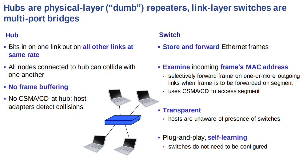
6.4.3 Link-Layer Switches


6.7 Retrospective: A Day in the Life of a Web Page Request
6.7.1 Getting Started: DHCP, UDP, IP, and Ethernet 6.7.2 Still Getting Started: DNS and ARP 6.7.3 Still Getting Started: Intra-Domain Routing to the DNS Server 6.7.4 Web Client-Server Interaction: TCP and HTTP
Summary